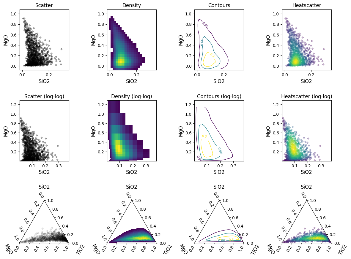
Heatscatter Plots

While density() plots are useful summary visualizations for large datasets, scatterplots are more precise and retain all spatial information (although they can get crowded).

A scatter plot where individual points are coloured by data density in some respects represents the best of both worlds. A version inspired by similar existing visualisations is implemented with heatscatter().

import matplotlib.pyplot as plt
import numpy as np
import pandas as pd

from pyrolite.plot import pyroplot

np.random.seed(12)

First we’ll create some example data

from pyrolite.util.synthetic import normal_frame, random_cov_matrix

df = normal_frame(
    size=1000,
    cov=random_cov_matrix(sigmas=np.random.rand(4) * 2, dim=4, seed=12),
    seed=12,
)

We can compare a minimal heatscatter() plot to other visualisations for the same data:

from pyrolite.util.plot.axes import share_axes

fig, ax = plt.subplots(3, 4, figsize=(12, 9))

ax = ax.flat
share_axes(ax[:4], which="xy")
share_axes(ax[4:8], which="xy")
share_axes(ax[8:], which="xy")

contours = [0.95, 0.66, 0.3]
bivar = ["SiO2", "MgO"]
trivar = ["SiO2", "MgO", "TiO2"]
# linear-scaled comparison
df.loc[:, bivar].pyroplot.scatter(ax=ax[0], c="k", s=10, alpha=0.3)
df.loc[:, bivar].pyroplot.density(ax=ax[1])
df.loc[:, bivar].pyroplot.density(ax=ax[2], contours=contours)
df.loc[:, bivar].pyroplot.heatscatter(ax=ax[3], s=10, alpha=0.3)
# log-log plots
df.loc[:, bivar].pyroplot.scatter(ax=ax[4], c="k", s=10, alpha=0.3)
df.loc[:, bivar].pyroplot.density(ax=ax[5], logx=True, logy=True)
df.loc[:, bivar].pyroplot.density(ax=ax[6], contours=contours, logx=True, logy=True)
df.loc[:, bivar].pyroplot.heatscatter(ax=ax[7], s=10, alpha=0.3, logx=True, logy=True)
# ternary plots
df.loc[:, trivar].pyroplot.scatter(ax=ax[8], c="k", s=10, alpha=0.1)
df.loc[:, trivar].pyroplot.density(ax=ax[9], bins=100)
df.loc[:, trivar].pyroplot.density(ax=ax[10], contours=contours, bins=100)
df.loc[:, trivar].pyroplot.heatscatter(ax=ax[11], s=10, alpha=0.3, renorm=True)
fig.subplots_adjust(hspace=0.4, wspace=0.4)

titles = ["Scatter", "Density", "Contours", "Heatscatter"]
for t, a in zip(titles + [i + " (log-log)" for i in titles], ax):
    a.set_title(t)
plt.tight_layout()