Log Ratio Means

import matplotlib.pyplot as plt
import numpy as np
import pandas as pd

import pyrolite.comp
from pyrolite.comp.codata import ILR, close, inverse_ILR
from pyrolite.plot import pyroplot
from pyrolite.util.synthetic import random_cov_matrix


np.random.seed(82)

def random_compositional_trend(m1, m2, c1, c2, resolution=20, size=1000):
    """
    Generate a compositional trend between two compositions with independent
    variances.
    """
    # generate means intermediate between m1 and m2
    mv = np.vstack([ILR(close(m1)).reshape(1, -1), ILR(close(m2)).reshape(1, -1)])
    ms = np.apply_along_axis(lambda x: np.linspace(*x, resolution), 0, mv)
    # generate covariance matricies intermediate between c1 and c2
    cv = np.vstack([c1.reshape(1, -1), c2.reshape(1, -1)])
    cs = np.apply_along_axis(lambda x: np.linspace(*x, resolution), 0, cv)
    cs = cs.reshape(cs.shape[0], *c1.shape)
    # generate samples from each
    samples = np.vstack(
        [
            np.random.multivariate_normal(m.flatten(), cs[ix], size=size // resolution)
            for ix, m in enumerate(ms)
        ]
    )
    # combine together.
    return inverse_ILR(samples)

First we create an array of compositions which represent a trend.

m1, m2 = np.array([[0.3, 0.1, 2.1]]), np.array([[0.5, 2.5, 0.05]])
c1, c2 = (
    random_cov_matrix(2, sigmas=[0.15, 0.05]),
    random_cov_matrix(2, sigmas=[0.05, 0.2]),
)

trend = pd.DataFrame(
    random_compositional_trend(m1, m2, c1, c2, resolution=100, size=5000),
    columns=["A", "B", "C"],
)

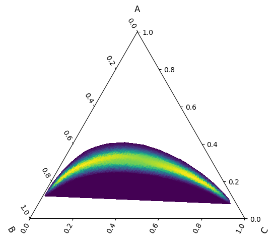
We can visualise this compositional trend with a density plot.

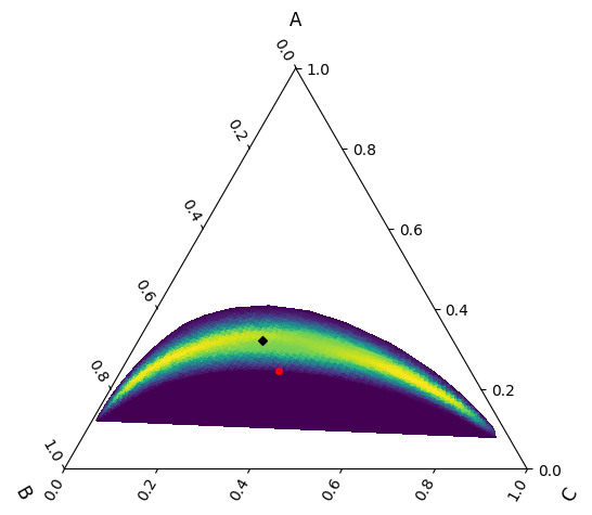
ax = trend.pyroplot.density(mode="density", bins=100)
plt.show()

First we can see where the geometric mean would fall:

geomean = trend.mean(axis=0).to_frame().T
ax = geomean.pyroplot.scatter(ax=ax, marker="o", color="r", zorder=2, label="GeoMean")
plt.show()

Finally, we can also see where the logratio mean would fall:

ILRmean = trend.pyrocomp.logratiomean(transform="ILR")
ax = ILRmean.pyroplot.scatter(ax=ax, color="k", label="LogMean")
plt.show()