Spherical Coordinate Transformations

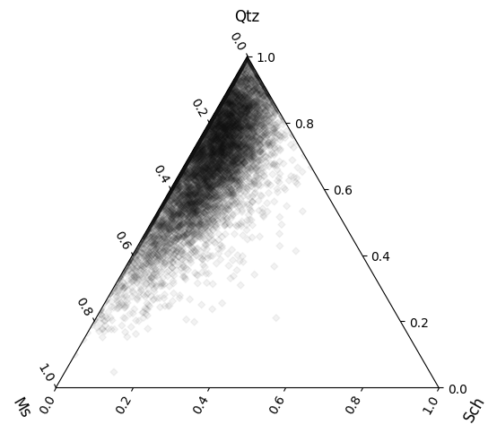
While logratio methods are typically more commonly used to deal with with compositional data, they are not infallible - their principal weakness is being able to deal with true zeros like we have the example dataset below. True zeros are common in mineralogical datasets, and are possible in geochemical datasets to some degree (at least at the level of atom counting..).

An alternative to this is to use a spherical coordinate transform to handle our compositional data. This typically involves treating each covariate as a separate dimension/axis and each composition as a unit vector in this space. The transformation invovles the iterative calculation of an angular representeation of these vectors. \(N\)-dimensional vectors transformed to \(N-1\) dimensional angular equivalents (as the first angle is that between the first axis and the second). At least two variants of this type of transformation exist - a spherical cosine method and a spherical sine method; these are complementary and the sine method is used here (where angles close to \(\pi / 2\) represent close to zero abundance, and angles closer to zero/aligning with the repsective component axis represent higher abundances). See below for an example of this demonstrated graphically.

First let’s create some example mineralogical abundance data, where at least one of the minerals might occasionally have zero abundance:

import numpy as np

from pyrolite.util.synthetic import normal_frame

comp = normal_frame(
    columns=["Ab", "Qtz", "Ms", "Sch"],
    mean=[0.5, 1, 0.3, 0.05],
    cov=np.eye(3) * np.array([0.02, 0.5, 0.5]),
    size=10000,
    seed=145,
)
comp += 0.05 * np.random.randn(*comp.shape)
comp[comp <= 0] = 0
comp = comp.pyrocomp.renormalise(scale=1)

We can quickly visualise this to see that it does indeed have some true zeros:

import matplotlib.pyplot as plt

comp[["Qtz", "Ms", "Sch"]].pyroplot.scatter(alpha=0.05, c="k")
plt.show()

The spherical coordinate transform functions can be found within pyrolite.comp.codata, but can also be accessed from the pyrocomp dataframe accessor:

import pyrolite.comp

angles = comp.pyrocomp.sphere()
angles.head()

	θ_Qtz	θ_Ms	θ_Sch
0	0.588	0.919	1.380
1	0.734	1.205	1.444
2	0.583	1.096	1.571
3	0.756	1.308	1.247
4	0.644	1.266	1.247

The inverse function can be accessed in the same way:

inverted_angles = angles.pyrocomp.inverse_sphere()
inverted_angles.head()

	Ab	Qtz	Ms	Sch
0	0.187	0.422	0.354	3.603e-02
1	0.385	0.473	0.126	1.600e-02
2	0.240	0.551	0.209	3.749e-33
3	0.395	0.443	0.061	1.010e-01
4	0.295	0.523	0.081	1.013e-01

We can see that the inverted angles are within precision of the original composition we used:

np.isclose(inverted_angles, comp.values).all()

True

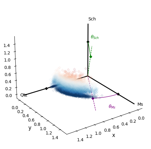
To better understand what’s going on here, visualising our data is often the best first step. Below we use a helper fucntion from pyrolite.util.plot.helpers to create a 3D axis on which to plot our angular data.

from pyrolite.plot.color import process_color
from pyrolite.util.plot.helpers import init_spherical_octant

ax = init_spherical_octant(labels=[c[2:] for c in angles.columns], figsize=(6, 6))

# here we can color the points by the angle from the Schorl axis
colors = process_color(angles["θ_Sch"], cmap="RdBu", alpha=0.1)["c"]
ax.scatter(*np.sqrt(comp.values[:, 1:]).T, c=colors)
plt.show()

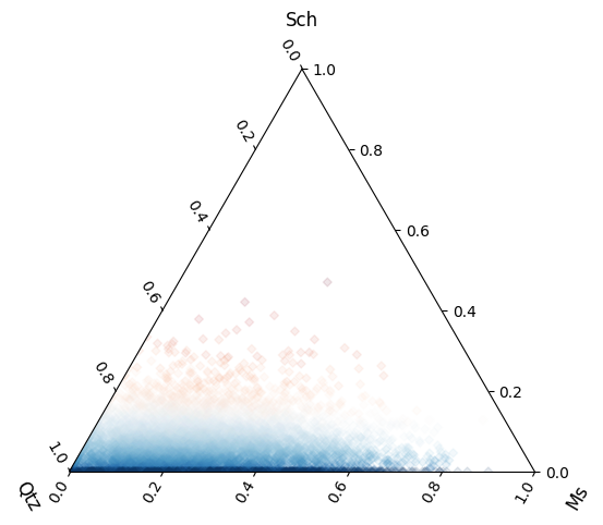
We can compare this to the equivalent ternary projection of our data; note we need to reorder some columns in order to make this align in the same way:

tcolumns = np.array([c[2:] for c in angles.columns])[[2, 0, 1]]
comp[tcolumns].pyroplot.scatter(c=colors)
plt.show()