TAS Classifier

Some simple discrimination methods are implemented, including the Total Alkali-Silica (TAS) classification.

import matplotlib.pyplot as plt
import numpy as np
import pandas as pd

from pyrolite.util.classification import TAS
from pyrolite.util.synthetic import normal_frame, random_cov_matrix

We’ll first generate some synthetic data to play with:

df = (
    normal_frame(
        columns=["SiO2", "Na2O", "K2O", "Al2O3"],
        mean=[0.5, 0.04, 0.05, 0.4],
        size=100,
        seed=49,
    )
    * 100
)

df.head(3)

	SiO2	Na2O	K2O	Al2O3
0	48.598	3.834	4.695	42.873
1	50.096	3.960	5.196	40.747
2	51.382	4.126	5.181	39.311

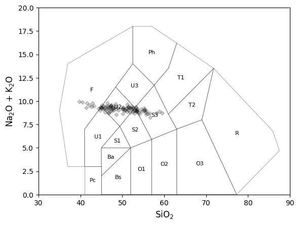
We can visualise how this chemistry corresponds to the TAS diagram:

df["Na2O + K2O"] = df["Na2O"] + df["K2O"]
cm = TAS()

fig, ax = plt.subplots(1)
cm.add_to_axes(ax, alpha=0.5, linewidth=0.5, zorder=-1, add_labels=True)
df[["SiO2", "Na2O + K2O"]].pyroplot.scatter(ax=ax, c="k", alpha=0.2, axlabels=False)
plt.show()

We can now classify this data according to the fields of the TAS diagram, and add this as a column to the dataframe. Similarly, we can extract which rock names the TAS fields correspond to:

df["TAS"] = cm.predict(df)
df["Rocknames"] = df.TAS.apply(lambda x: cm.fields.get(x, {"name": None})["name"])
df["Rocknames"].sample(10)  # randomly check 10 sample rocknames

78    [Phonotephrite, Foid Monzodiorite]
2     [Phonotephrite, Foid Monzodiorite]
56    [Phonotephrite, Foid Monzodiorite]
41    [Phonotephrite, Foid Monzodiorite]
93    [Phonotephrite, Foid Monzodiorite]
60    [Phonotephrite, Foid Monzodiorite]
61    [Phonotephrite, Foid Monzodiorite]
47    [Phonotephrite, Foid Monzodiorite]
4         [Trachy-\nandesite, Monzonite]
12        [Trachy-\nandesite, Monzonite]
Name: Rocknames, dtype: object

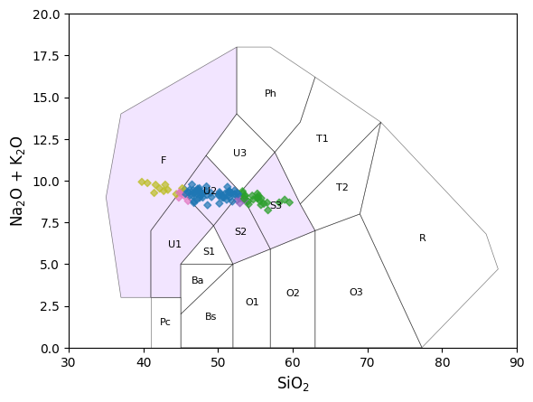
We could now take the TAS classes and use them to colorize our points for plotting on the TAS diagram, or more likely, on another plot. Here the relationship to the TAS diagram is illustrated, coloring also the populated fields:

fig, ax = plt.subplots(1)

cm.add_to_axes(ax, alpha=0.5, linewidth=0.0, zorder=-2, add_labels=False,
               which_ids=np.unique(df["TAS"]), fill=True, facecolor=[0.9, 0.8, 1.0])
cm.add_to_axes(ax, alpha=0.5, linewidth=0.5, zorder=-1, add_labels=True)
df[["SiO2", "Na2O + K2O"]].pyroplot.scatter(ax=ax, c=df["TAS"], alpha=0.7, axlabels=False)

<Axes: xlabel='SiO$_2$', ylabel='Na$_2$O + K$_2$O'>

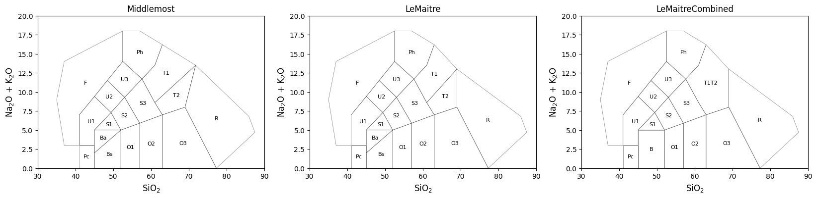
Variations of the Diagram

To use a different variation of the TAS diagram, you can pass the relevant keyword which_model allowing you to access the other available variants.

Currently, the Le Bas/Le Maitre alternative and a T1-T2 combined variant of it are available as alternatives to the Middlemost version. Each of these can be used as a classifier model as for the default above.

fig, ax = plt.subplots(1, 3, figsize=(20, 4))
for a, model in zip(ax, ["Middlemost", "LeMaitre", "LeMaitreCombined"]):
    a.set_title(model if model is not None else "")
    cm = TAS(which_model=model)
    cm.add_to_axes(a, alpha=0.5, linewidth=0.5, add_labels=True)
plt.show()

References & Citation

For a few references on the TAS diagram as used here:

Middlemost, E. A. K. (1994).Naming materials in the magma/igneous rock system. Earth-Science Reviews, 37(3), 215–224. doi: 10.1016/0012-8252(94)90029-9.

Le Bas, M.J., Le Maitre, R.W., Woolley, A.R. (1992). The construction of the Total Alkali-Silica chemical classification of volcanic rocks. Mineralogy and Petrology 46, 1–22. doi: 110.1007/BF01160698.

Le Maitre, R.W. (2002). Igneous Rocks: A Classification and Glossary of Terms : Recommendations of International Union of Geological ciences Subcommission on the Systematics of Igneous Rocks. Cambridge University Press, 236pp. doi: 10.1017/CBO9780511535581.