Lattice Strain Calculations

Note

This example follows that given during a Institute of Advanced Studies Masterclass with Jon Blundy at the University of Western Australia on the 29^th April 2019, and is used here with permission.

Pyrolite includes a function for calculating relative lattice strain [1], which together with the tables of Shannon ionic radii and Young’s modulus approximations for silicate and oxide cationic sites enable relatively simple calculation of ionic partitioning in common rock forming minerals.

This example below uses previously characterised calcium and sodium partition coefficients between plagioclase (\(CaAl_2Si_2O_8 - NaAlSi_3O8\)) and silicate melt to estimate partitioning for other cations based on their ionic radii.

A model parameterised using sodium and calcium partition coefficients [2] is then used to estimate the partitioning for lanthanum into the trivalent site (largely occupied by \(Al^{3+}\)), and extended to other trivalent cations (here, the Rare Earth Elements). The final section of the example highlights the mechanism which generates plagioclase’s hallmark ‘europium anomaly’, and the effects of variable europium oxidation state on bulk europium partitioning.

import matplotlib.pyplot as plt
import numpy as np

from pyrolite.geochem.ind import REE, get_ionic_radii
from pyrolite.mineral.lattice import strain_coefficient

First, we need to define some of the necessary parameters including temperature, the Young’s moduli for the \(X^{2+}\) and \(X^{3+}\) sites in plagioclase (\(E_2\), \(E_3\)), and some reference partition coefficients and radii for calcium and sodium:

D_Na = 1.35  # Partition coefficient Plag-Melt
D_Ca = 4.1  # Partition coefficient Plag-Melt
Tc = 900  # Temperature, °C
Tk = Tc + 273.15  # Temperature, K
E_2 = 120 * 10**9  # Youngs modulus for 2+ site, Pa
E_3 = 135 * 10**9  # Youngs modulus for 3+ site, Pa
r02, r03 = 1.196, 1.294  # fictive ideal cation radii for these sites
rCa = get_ionic_radii("Ca", charge=2, coordination=8)
rLa = get_ionic_radii("La", charge=3, coordination=8)

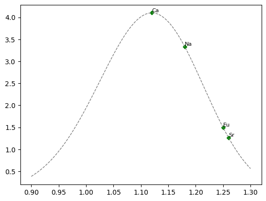
We can calculate and plot the partitioning of \(X^{2+}\) cations relative to \(Ca^{2+}\) at a given temperature using their radii and the lattice strain function:

fontsize = 8
fig, ax = plt.subplots(1)
ax.set(ylabel="$D_X$", xlabel="Radii ($\AA$)", yscale="log")
site2labels = ["Na", "Ca", "Eu", "Sr"]
# get the Shannon ionic radii for the elements in the 2+ site
site2radii = [
    get_ionic_radii("Na", charge=1, coordination=8),
    *get_ionic_radii(["Ca", "Eu", "Sr"], charge=2, coordination=8),
]
# plot the relative paritioning curve for cations in the 2+ site
site2Ds = D_Ca * np.array(
    [strain_coefficient(rCa, rx, r0=r02, E=E_2, T=Tk) for rx in site2radii]
)
ax.scatter(site2radii, site2Ds, color="g", label="$X^{2+}$ Cations")
# create an index of radii, and plot the relative paritioning curve for the site
xs = np.linspace(0.9, 1.3, 200)
curve2Ds = D_Ca * strain_coefficient(rCa, xs, r0=r02, E=E_2, T=Tk)
ax.plot(xs, curve2Ds, color="0.5", ls="--")
# add the element labels next to the points
for l, r, d in zip(site2labels, site2radii, site2Ds):
    ax.annotate(
        l, xy=(r, d), xycoords="data", ha="left", va="bottom", fontsize=fontsize
    )
fig

/home/docs/checkouts/readthedocs.org/user_builds/pyrolite/checkouts/main/docs/source/gallery/examples/geochem/mineral_lattice.py:56: SyntaxWarning: invalid escape sequence '\A'
  ax.set(ylabel="$D_X$", xlabel="Radii ($\AA$)", yscale="log")

<Figure size 640x480 with 1 Axes>

When it comes to estimating the partitioning of \(X^{3+}\) cations, we’ll need a reference point - here we’ll use \(D_{La}\) to calculate relative partitioning of the other Rare Earth Elements, although you may have noticed it is not defined above. Through a handy relationship, we can estimate \(D_{La}\) based on the easier measured \(D_{Ca}\), \(D_{Na}\) and temperature [2]:

D_La = (D_Ca**2 / D_Na) * np.exp((529 / Tk) - 3.705)
D_La  # 0.48085

np.float64(0.48084614946362086)

Now \(D_{La}\) is defined, we can use it as a reference for the other REE:

site3labels = REE(dropPm=True)
# get the Shannon ionic radii for the elements in the 3+ site
site3radii = get_ionic_radii([x for x in REE(dropPm=True)], charge=3, coordination=8)
site3Ds = D_La * np.array(
    [strain_coefficient(rLa, rx, r0=r03, E=E_3, T=Tk) for rx in site3radii]
)
# plot the relative paritioning curve for cations in the 3+ site
ax.scatter(site3radii, site3Ds, color="purple", label="$X^{3+}$ Cations")
# plot the relative paritioning curve for the site
curve3Ds = D_La * strain_coefficient(rLa, xs, r0=r03, E=E_3, T=Tk)
ax.plot(xs, curve3Ds, color="0.5", ls="--")
# add the element labels next to the points
for l, r, d in zip(site3labels, site3radii, site3Ds):
    ax.annotate(
        l, xy=(r, d), xycoords="data", ha="right", va="bottom", fontsize=fontsize
    )
fig

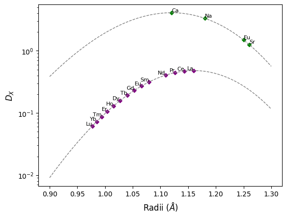
<Figure size 640x480 with 1 Axes>

As europium is commonly present as a mixture of both \(Eu^{2+}\) and \(Eu^{3+}\), the effective partitioning of Eu will be intermediate between that of \(D_{Eu^{2+}}`and :math:`D_{Eu^{3+}}\). Using a 60:40 mixture of \(Eu^{3+}\) : \(Eu^{2+}\) as an example, this effective partition coefficient can be calculated:

X_Eu3 = 0.6
# calculate D_Eu3 relative to D_La
D_Eu3 = D_La * strain_coefficient(
    rLa, get_ionic_radii("Eu", charge=3, coordination=8), r0=r03, E=E_3, T=Tk
)
# calculate D_Eu2 relative to D_Ca
D_Eu2 = D_Ca * strain_coefficient(
    rCa, get_ionic_radii("Eu", charge=2, coordination=8), r0=r02, E=E_2, T=Tk
)
# calculate the effective parition coefficient
D_Eu = (1 - X_Eu3) * D_Eu2 + X_Eu3 * D_Eu3
# show the effective partition coefficient relative to the 2+ and 3+ endmembers
radii, ds = (
    [get_ionic_radii("Eu", charge=c, coordination=8) for c in [3, 3, 2, 2]],
    [D_Eu3, D_Eu, D_Eu, D_Eu2],
)
ax.plot(radii, ds, ls="--", color="0.9", label="Effective $D_{Eu}$", zorder=-1)
ax.legend(bbox_to_anchor=(1.05, 1))
fig

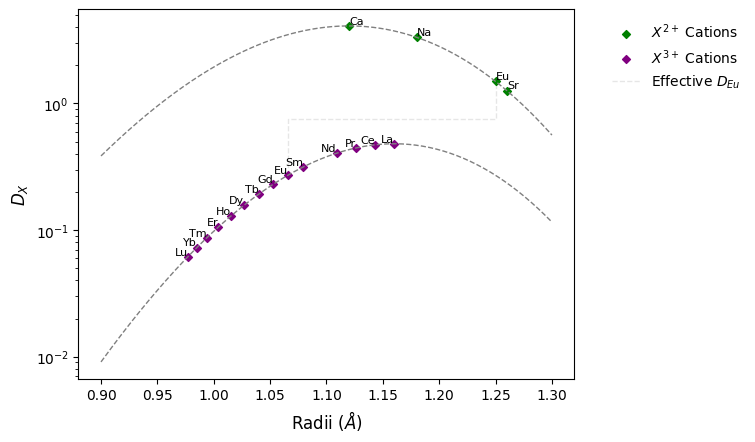
<Figure size 640x480 with 1 Axes>

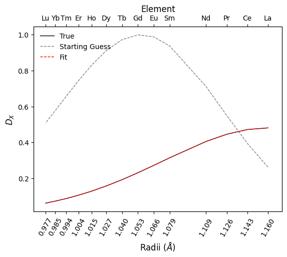
Fitting Lattice Strain Models

Given the lattice strain model and a partitioning profile (for e.g. REE data), we can also fit a model to a given curve; here we fit to our REE data above, for which we have some known parameters to compare to. Note that this uses the youngs modulus approximation behind the scenes where it isn’t provided:

from pyrolite.mineral.lattice import fit_lattice_strain, youngs_modulus_approximation

t0 = 273.15 + 700  # estimated temperature
_ri, _tk, _D = fit_lattice_strain(site3radii, site3Ds, z=3, t0=t0)

We can compare the results of this fit to our source parameters - the ionic radius of La, 900°C and estimated \(D_{La}\) - note that the temperature isn’t being fit well here, but the other parameters are recovered reasonably well:

import pandas as pd

pd.DataFrame(
    [(_ri, rLa), (Tk, _tk), (D_La, _D)],
    index=["radii", "T", "D"],
    columns=["Source Parameters", "Fit Parameters"],
).T

	radii	T	D
Source Parameters	1.16	1173.150	0.481
Fit Parameters	1.16	1581.532	0.481

From this point, we could We can also compare the curves visually:

from pyrolite.plot.spider import REE_v_radii

ax = REE_v_radii(index="radii")
ax.set(ylabel="$D_X$", xlabel="Radii ($\AA$)")

ax.plot(site3radii, site3Ds, label="True", color="k")

r0 = site3radii.mean()
starting_guess = strain_coefficient(
    r0, site3radii, r0=r0, z=3, T=t0, E=youngs_modulus_approximation(3, r0)
)
ax.plot(site3radii, starting_guess, label="Starting Guess", ls="--", color="0.5")

fit_curve = _D * strain_coefficient(
    _ri, site3radii, r0=_ri, T=_tk, z=3, E=youngs_modulus_approximation(3, _ri)
)
ax.plot(site3radii, fit_curve, color="r", ls="--", label="Fit")

ax.legend()
ax.figure

/home/docs/checkouts/readthedocs.org/user_builds/pyrolite/checkouts/main/docs/source/gallery/examples/geochem/mineral_lattice.py:164: SyntaxWarning: invalid escape sequence '\A'
  ax.set(ylabel="$D_X$", xlabel="Radii ($\AA$)")

<Figure size 640x480 with 2 Axes>

See also

Examples:

Shannon Radii, REE Radii Plot

Functions:

strain_coefficient(), youngs_modulus_approximation(), fit_lattice_strain() get_ionic_radii()

References

[1]

Blundy, J., Wood, B., 1994. Prediction of crystal–melt partition coefficients from elastic moduli. Nature 372, 452. doi: 10.1038/372452A0

[2] (1,2)

Dohmen, R., Blundy, J., 2014. A predictive thermodynamic model for element partitioning between plagioclase and melt as a function of pressure, temperature and composition. American Journal of Science 314, 1319–1372. doi: 10.2475/09.2014.04