lambdas: Parameterising REE Profiles
Orthogonal polynomial decomposition can be used for dimensional reduction of smooth function over an independent variable, producing an array of independent values representing the relative weights for each order of component polynomial. This is an effective method to parameterise and compare the nature of smooth profiles.
In geochemistry, the most applicable use case is for reduction Rare Earth Element (REE) profiles. The REE are a collection of elements with broadly similar physicochemical properties (the lanthanides), which vary with ionic radii. Given their similar behaviour and typically smooth function of normalised abundance vs. ionic radii, the REE profiles and their shapes can be effectively parameterised and dimensionally reduced (14 elements summarised by 3-4 shape parameters).
Note
A publication discussing this implementation of lambdas together with fitting tetrads for REE patterns has been published in Mathematical Geosciences!
Here we generate some example data, reduce these to lambda values, and visualise the results.
import matplotlib.pyplot as plt
import numpy as np
import pandas as pd

import pyrolite.plot


np.random.seed(82)
First we’ll generate some example synthetic data based around Depleted MORB Mantle:
from pyrolite.util.synthetic import example_spider_data

df = example_spider_data(
    noise_level=0.05,
    size=100,
    start="DMM_WH2005",
    norm_to="Chondrite_PON",
    offsets={"Eu": 0.2},
).pyrochem.REE.pyrochem.denormalize_from("Chondrite_PON")
df.head(2)
Let’s have a quick look at what this REE data looks like normalized to Primitive Mantle:
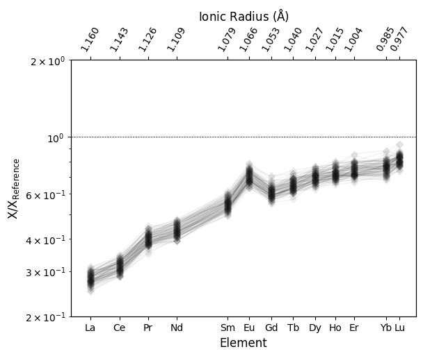
From this REE data we can fit a series of orthogonal polynomials, and subsequently used the regression coefficients (‘lambdas’) as a parameterisation of the REE pattern/profile:
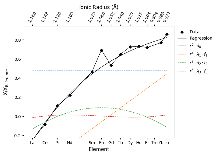
So what’s actually happening here? To get some idea of what these λ coefficients
correspond to, we can pull this process apart and visualise our REE profiles as
the sum of the series of orthogonal polynomial components of increasing order.
As lambdas represent the coefficients for the regression of log-transformed normalised
data, to compare the polynomial components and our REE profile we’ll first need to
normalize it to the appropriate composition (here "ChondriteREE_ON") before
taking the logarithm.
With our data, we’ve then fit a function of ionic radius with the form \(f(r) = \lambda_0 + \lambda_1 f_1 + \lambda_2 f_2 + \lambda_3 f_3...\) where the polynomial components of increasing order are \(f_1 = (r - \beta_0)\), \(f_2 = (r - \gamma_0)(r - \gamma_1)\), \(f_3 = (r - \delta_0)(r - \delta_1)(r - \delta_2)\) and so on. The parameters \(\beta\), \(\gamma\), \(\delta\) are pre-computed such that the polynomial components are indeed independent. Here we can visualise how these polynomial components are summed to produce the regressed profile, using the last REE profile we generated above as an example:
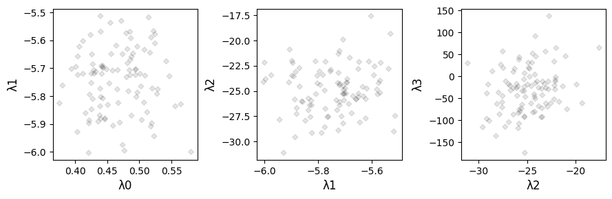
Now that we’ve gone through a brief introduction to how the lambdas are generated, let’s quickly check what the coefficient values themselves look like:
fig, ax = plt.subplots(1, 3, figsize=(9, 3))
for ix in range(ls.columns.size - 1):
    ls[ls.columns[ix : ix + 2]].pyroplot.scatter(ax=ax[ix], alpha=0.1, c="k")

plt.tight_layout()
/home/docs/checkouts/readthedocs.org/user_builds/pyrolite/checkouts/main/docs/source/gallery/examples/geochem/lambdas.py:97: RuntimeWarning: More than 20 figures have been opened. Figures created through the pyplot interface (`matplotlib.pyplot.figure`) are retained until explicitly closed and may consume too much memory. (To control this warning, see the rcParam `figure.max_open_warning`). Consider using `matplotlib.pyplot.close()`.
  fig, ax = plt.subplots(1, 3, figsize=(9, 3))
But what do these parameters correspond to? From the deconstructed orthogonal polynomial above, we can see that \(\lambda_0\) parameterises relative enrichment (this is the mean value of the logarithm of Chondrite-normalised REE abundances), \(\lambda_1\) parameterises a linear slope (here, LREE enrichment), and higher order terms describe curvature of the REE pattern. Through this parameterisation, the REE profile can be effectively described and directly linked to geochemical processes. While the amount of data we need to describe the patterns is lessened, the values themselves are more meaningful and readily used to describe the profiles and their physical significance.
The visualisation of \(\lambda_1\)-\(\lambda_2\) can be particularly useful where you’re trying to compare REE profiles.
We’ve used a synthetic dataset here which is by design approximately normally distributed, so the values themeselves here are not particularly revealing, but they do illustrate the expected mangitudes of values for each of the parameters.
Dealing With Anomalies
Note that we’ve not used Eu in this regression - Eu anomalies are a deviation from
the ‘smooth profile’ we need to use this method. Consider this if your data might also
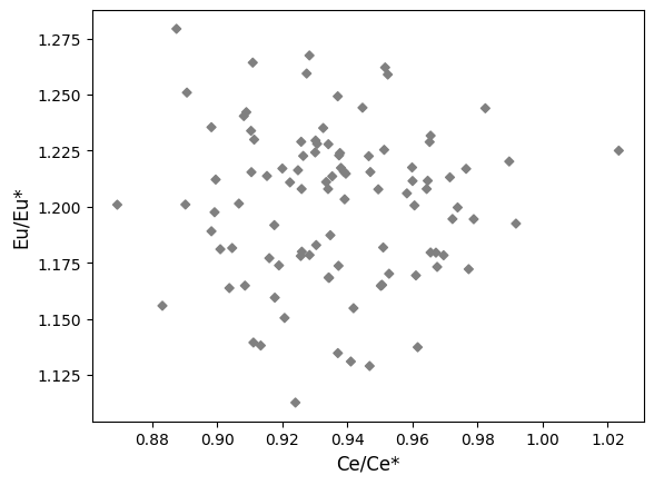
exhibit significant Ce anomalies, you might need to exclude this data. For convenience
there is also functionality to calculate anomalies derived from the orthogonal
polynomial fit itself (rather than linear interpolation methods). Below we use the
anomalies keyword argument to also calculate the \(\frac{Ce}{Ce*}\)
and \(\frac{Eu}{Eu*}\) anomalies (note that these are excluded from the fit):
ls_anomalies = df.pyrochem.lambda_lnREE(anomalies=["Ce", "Eu"])
ax = ls_anomalies.iloc[:, -2:].pyroplot.scatter(color="0.5")
plt.show()
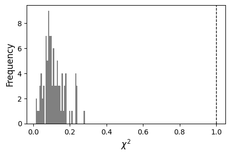
Coefficient Uncertainties and Fit Quality
In order to determine the relative significance of the parameterisation and ‘goodness of fit’, the functions are able to estimate uncertainties on the returned coefficients (lambdas and taus) and will also return the chi-square value (\(\chi^2\); equivalent to the MSWD) where requested. This will be appended to the end of the dataframe. Note that if you do not supply an estimate of observed value uncertainties a default of 1% of the log-mean will be used.
To append the reduced chi-square for each row, the keyword argument
add_X2=True can be used; here we’ve estimated 10% uncertainty on the
REE:
ls = df.pyrochem.lambda_lnREE(add_X2=True, sigmas=0.1, anomalies=["Eu", "Ce"])
ls.columns
Index(['λ0', 'λ1', 'λ2', 'λ3', 'X2', 'Eu/Eu*', 'Ce/Ce*'], dtype='str')
We can have a quick look at the \(\chi^2\) values look like for the synthetic dataset, given the assumed 10% uncertainties. While the fit appears reasonable for a good fraction of the dataset (~2 and below), for some rows it is notably worse:
/home/docs/checkouts/readthedocs.org/user_builds/pyrolite/checkouts/main/docs/source/gallery/examples/geochem/lambdas.py:159: SyntaxWarning: invalid escape sequence '\c'
  ax.set(xlabel="$\chi^2$")
We can also examine the estimated uncertainties on the coefficients from the fit
by adding the keyword argument add_uncertainties=True (note: these do not
explicitly propagate observation uncertainties):
ls = df.pyrochem.lambda_lnREE(add_uncertainties=True)
ls.columns
Index(['λ0', 'λ1', 'λ2', 'λ3', 'λ0_σ', 'λ1_σ', 'λ2_σ', 'λ3_σ'], dtype='str')
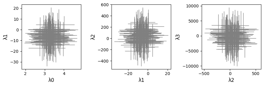
Notably, on the scale of natural dataset variation, these uncertainties may end up being smaller than symbol sizes. If your dataset happened to have a great deal more noise, you may happen to see them - for demonstration purposes we can generate a noiser dataset and have a quick look at what these uncertainties could look like:
ls = (df + 3 * np.exp(np.random.randn(*df.shape))).pyrochem.lambda_lnREE(
    add_uncertainties=True
)
With this ‘noisy’ dataset, we can see some of the errorbars:
fig, ax = plt.subplots(1, 3, figsize=(9, 3))
ax = ax.flat
dc = ls.columns.size // 2
for ix, a in enumerate(ls.columns[:3]):
    i0, i1 = ix, ix + 1
    ax[ix].set(xlabel=ls.columns[i0], ylabel=ls.columns[i1])
    ax[ix].errorbar(
        ls.iloc[:, i0],
        ls.iloc[:, i1],
        xerr=ls.iloc[:, i0 + dc] * 2,
        yerr=ls.iloc[:, i1 + dc] * 2,
        ls="none",
        ecolor="0.5",
        markersize=1,
        color="k",
    )
plt.tight_layout()
plt.show()
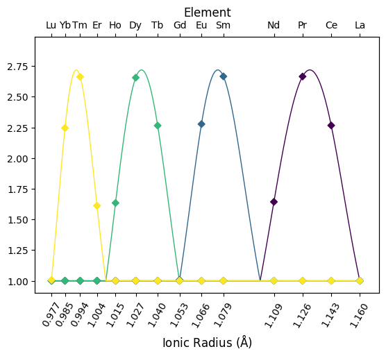
Fitting Tetrads
In addition to fitting orothogonal polynomial functions, the ability to fit tetrad functions has also recently been added. This supplements the \(\lambda\) coefficients with \(\tau\) coefficients which describe subtle electronic configuration effects affecting sequential subsets of the REE. Below we plot four profiles - each describing only a single tetrad - to illustrate the shape of these function components. Note that these are functions of \(z\), and are here transformed to plot against radii.
from pyrolite.util.lambdas.plot import plot_profiles

# let's first create some synthetic pattern parameters
# we want lambdas to be zero, and each of the tetrads to be shown in only one pattern
lambdas = np.zeros((4, 5))
tetrads = np.eye(4)
# putting it together to generate four sets of combined parameters
fit_parameters = np.hstack([lambdas, tetrads])

ax = plot_profiles(
    fit_parameters,
    tetrads=True,
    color=np.arange(4),
)
plt.show()
In order to also fit these function components, you can pass the keyword argument
fit_tetrads=True to lambda_lnREE() and
related functions:
We can see that the four extra \(\tau\) Parameters have been appended to the right of the lambdas within the output:
lts.head(2)
from pyrolite.geochem.ind import REE
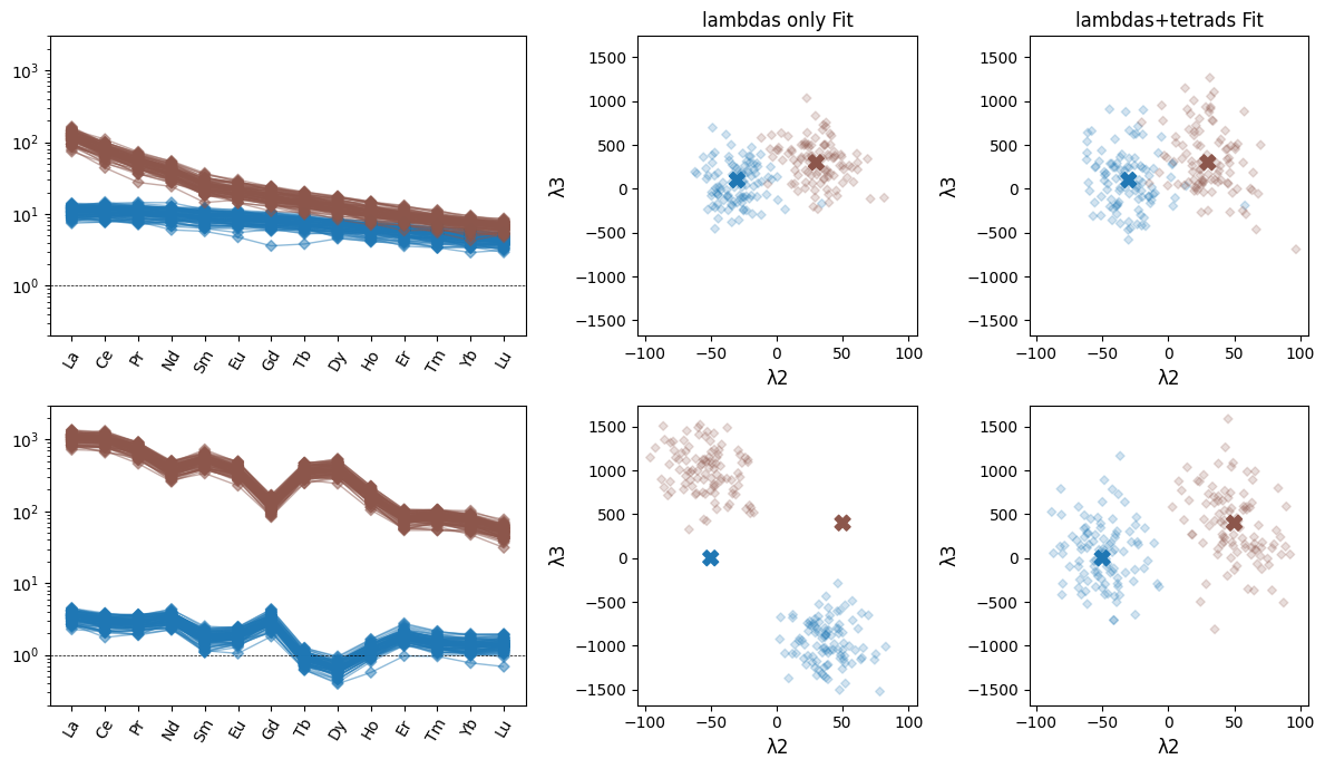
Below we’ll look at some of the potential issues of fitting lambdas and tetrads together - by examining the effects of i) fitting tetrads where there are none and ii) not fitting tetrads where they do indeed exist using some synthetic datasets.
from pyrolite.util.synthetic import example_patterns_from_parameters

ls = np.array(
    [
        [2, 5, -30, 100, -600, 0, 0, 0, 0],  # lambda-only
        [3, 15, 30, 300, 1500, 0, 0, 0, 0],  # lambda-only
        [1, 5, -50, 0, -1000, -0.3, -0.7, -1.4, -0.2],  # W-pattern tetrad
        [5, 15, 50, 400, 2000, 0.6, 1.1, 1.5, 0.3],  # M-pattern tetrad
    ]
)
# now we use these parameters to generate some synthetic log-scaled normalised REE
# patterns and add a bit of noise
pattern_df = pd.DataFrame(
    np.vstack([example_patterns_from_parameters(l, includes_tetrads=True) for l in ls]),
    columns=REE(),
)
# We can now fit these patterns and see what the effect of fitting and not-Fitting
# tetrads might look like in these (slightly extreme) cases:
fit_ls_only = pattern_df.pyrochem.lambda_lnREE(
    norm_to=None, degree=5, fit_tetrads=False
)
fit_ts = pattern_df.pyrochem.lambda_lnREE(norm_to=None, degree=5, fit_tetrads=True)
We can now examine what the differences between the fits are. Below we plot the four sets of synthetic REE patterns (lambda-only above and lamba+tetrad below) and examine the relative accuracy of fitting some of the higher order lambda parameters where tetrads are also fit:
from pyrolite.util.plot.axes import share_axes

x, y = 2, 3
categories = np.repeat(np.arange(ls.shape[0]), 100)
colors = np.array([str(ix) * 2 for ix in categories])
l_only = categories < 2

ax = plt.figure(figsize=(12, 7)).subplot_mosaic(
    """
    AAABBCC
    DDDEEFF
    """
)
share_axes([ax["A"], ax["D"]])
share_axes([ax["B"], ax["C"], ax["E"], ax["F"]])

ax["B"].set_title("lambdas only Fit")
ax["C"].set_title("lambdas+tetrads Fit")


for a, fltr in zip(["A", "D"], [l_only, ~l_only]):
    pattern_df.iloc[fltr, :].pyroplot.spider(
        ax=ax[a],
        label="True",
        unity_line=True,
        alpha=0.5,
        color=colors[fltr],
    )

for a, fltr in zip(["B", "E"], [l_only, ~l_only]):
    fit_ls_only.iloc[fltr, [x, y]].pyroplot.scatter(
        ax=ax[a],
        alpha=0.2,
        color=colors[fltr],
    )

for a, fltr in zip(["C", "F"], [l_only, ~l_only]):
    fit_ts.iloc[fltr, [x, y]].pyroplot.scatter(
        ax=ax[a],
        alpha=0.2,
        color=colors[fltr],
    )


true = pd.DataFrame(ls[:, [x, y]], columns=[fit_ls_only.columns[ix] for ix in [x, y]])
for ix, a in enumerate(["B", "C", "E", "F"]):
    true.iloc[np.array([ix < 2, ix < 2, ix >= 2, ix >= 2]), :].pyroplot.scatter(
        ax=ax[a],
        color=np.array([str(ix) * 2 for ix in np.arange(ls.shape[0] // 2)]),
        marker="X",
        s=100,
    )

plt.tight_layout()
plt.show()
More Advanced Customisation
Above we’ve used default parameterisations for calculating lambdas, but
pyrolite allows you to customise the parameterisation of both the orthogonal
polynomial components used in the fitting process as well as what data and algorithm
is used in the fit itself.
To exclude some elements from the fit (e.g. Eu which is excluded by default, and and potentially Ce), you can either i) filter the dataframe such that the columns aren’t passed, or ii) explicitly exclude them:
# filtering the dataframe first
target_columns = [i for i in df.columns if i not in ["Eu", "Ce"]]
ls_noEuCe_filtered = df[target_columns].pyrochem.lambda_lnREE()
# excluding some elements
ls_noEuCe_excl = df.pyrochem.lambda_lnREE(exclude=["Eu", "Ce"])

# quickly checking equivalence
np.allclose(ls_noEuCe_excl, ls_noEuCe_filtered)
True
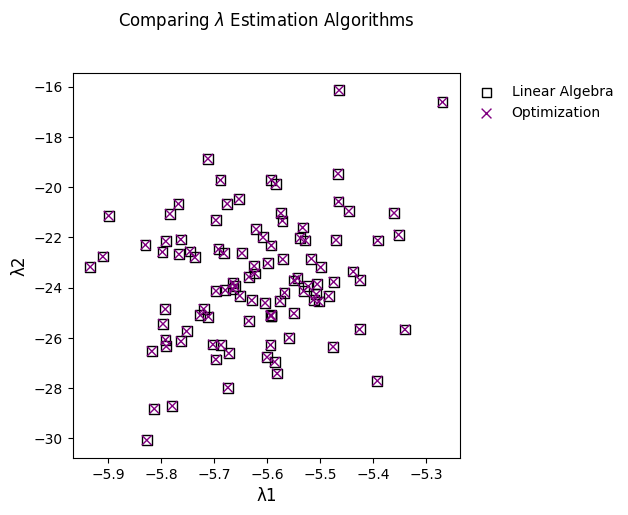
While the results should be numerically equivalent, pyrolite does provide
two algorithms for fitting lambdas. The first follows almost exactly the original
formulation (algorithm="ONeill"; this was translated from VBA), while the
second simply uses a numerical optimization routine from scipy to achieve the
same thing (algorithm="opt"; this is a fallback for where singular matricies
pop up):
To quickly demonstrate the equivalance, we can check numerically (to within 0.001%):
np.allclose(ls_linear, ls_opt, rtol=10e-5)
True
Or simply plot the results from both:
fig, ax = plt.subplots(1, figsize=(5, 5))
ax.set_title("Comparing $\lambda$ Estimation Algorithms", y=1.1)
ls_linear.iloc[:, 1:3].pyroplot.scatter(
    ax=ax, marker="s", c="k", facecolors="none", s=50, label="Linear Algebra"
)
ls_opt.iloc[:, 1:3].pyroplot.scatter(
    ax=ax, c="purple", marker="x", s=50, label="Optimization"
)
ax.legend()
plt.show()
/home/docs/checkouts/readthedocs.org/user_builds/pyrolite/checkouts/main/docs/source/gallery/examples/geochem/lambdas.py:372: SyntaxWarning: invalid escape sequence '\l'
  ax.set_title("Comparing $\lambda$ Estimation Algorithms", y=1.1)
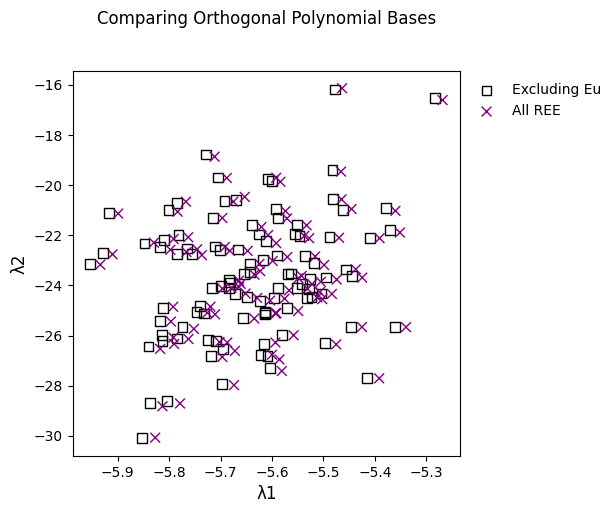
You can also use orthogonal polynomials defined over a different set of REE, by specifying the parameters using the keyword argument params:
# this is the original formulation from the paper, where Eu is excluded
ls_original = df.pyrochem.lambda_lnREE(params="ONeill2016")

# this uses a full set of REE
ls_fullREE_polynomials = df.pyrochem.lambda_lnREE(params="full")
Note that as of pyrolite v0.2.8, the original formulation is used by default,
but this will cease to be the case as of the following version, where the full set of
REE will instead be used to generate the orthogonal polynomials.
While the results are simlar, there are small differences. They’re typically less than 1%:
np.abs((ls_original / ls_fullREE_polynomials) - 1).max() * 100
λ0    8.265e-01
λ1    4.306e-01
λ2    7.584e-01
λ3    1.322e-06
dtype: float64
This can also be visualised:
fig, ax = plt.subplots(1, figsize=(5, 5))
ax.set_title("Comparing Orthogonal Polynomial Bases", y=1.1)
ls_original.iloc[:, 1:3].pyroplot.scatter(
    ax=ax, marker="s", c="k", facecolors="none", s=50, label="Excluding Eu"
)
ls_fullREE_polynomials.iloc[:, 1:3].pyroplot.scatter(
    ax=ax, c="purple", marker="x", s=50, label="All REE"
)
ax.legend()
plt.show()
References & Citation
For more on using orthogonal polynomials to describe geochemical pattern data, dig into the paper which introduced the method to geochemists:
O’Neill, H.S.C., 2016. The Smoothness and Shapes of Chondrite-normalized Rare Earth Element Patterns in Basalts. J Petrology 57, 1463–1508. doi: 10.1093/petrology/egw047.
If you’re using pyrolite’s implementation of lambdas in your research,
please consider citing a recent publication directly related to this:
Anenburg, M., & Williams, M. J. (2021). Quantifying the Tetrad Effect, Shape Components, and Ce–Eu–Gd Anomalies in Rare Earth Element Patterns. Mathematical Geosciences. doi: 10.1007/s11004-021-09959-5
See also
- Examples:
- Functions:
lambda_lnREE(),get_ionic_radii(),pyrolite.plot.pyroplot.REE()
Total running time of the script: (0 minutes 7.768 seconds)