One Way to Do Ternary Heatmaps

There are multiple ways you can acheive ternary heatmaps, but those based on the cartesian axes (e.g. a regularly spaced rectangular grid, or even a regularly spaced triangular grid) can result in difficulties and data misrepresentation.

Here we illustrate how the ternary heatmaps for pyrolite are constructed using an irregualr triangulated grid and log transforms, and how this avoids some of the potential issues of the methods mentioned above.

Let’s first get some data to deal with. mpltern has a conventient dataset which we can use here:

import numpy as np
import pandas as pd
from mpltern.ternary.datasets import get_scatter_points

np.random.seed(43)
df = pd.DataFrame(np.array([*get_scatter_points(n=80)]).T, columns=["A", "B", "C"])
df = df.loc[(df > 0.1).all(axis=1), :]

/home/docs/checkouts/readthedocs.org/user_builds/pyrolite/envs/develop/lib/python3.10/site-packages/mpltern/ternary/datasets.py:9: UserWarning: `mpltern.ternary.datasets.py` has been moved to `mpltern.datasets.py` and will be removed from the present directory in mpltern 0.6.0.
  warnings.warn(msg)

From this dataset we’ll generate a ternary_heatmap(), which is the basis for ternary density diagrams via density():

from pyrolite.comp.codata import ILR, inverse_ILR
from pyrolite.plot.density.ternary import ternary_heatmap

coords, H, data = ternary_heatmap(
    df.values,
    bins=10,
    mode="density",
    remove_background=True,
    transform=ILR,
    inverse_transform=inverse_ILR,
    grid_border_frac=0.2,
)

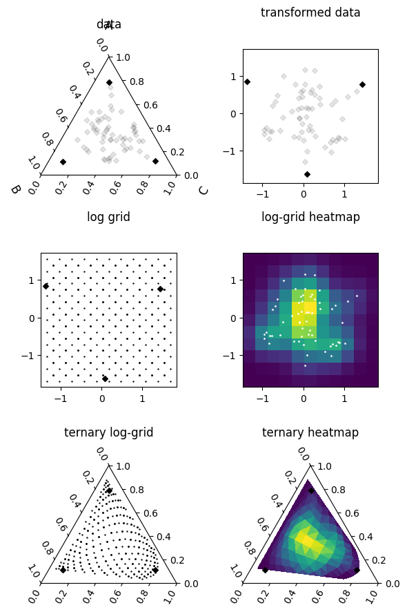
This function returns more than just the coordinates and histogram/density estimate, which will come in handy for exploring how it came together. The data variable here is a dictonary with contains the grids and coordiantes used to construct the histogram/density diagram. We can use these to show how the ternary log-grid is constructed, and then transformed back to ternary space before being triangulated and interpoalted for the ternary heatmap:

import matplotlib.pyplot as plt

import pyrolite.plot
from pyrolite.util.math import flattengrid
from pyrolite.util.plot.axes import axes_to_ternary, share_axes

fig, ax = plt.subplots(3, 2, figsize=(6, 9))
ax = ax.flat

share_axes([ax[1], ax[2], ax[3]])
ax = axes_to_ternary([ax[0], ax[4], ax[5]])

ax[0].set_title("data", y=1.2)
df.pyroplot.scatter(ax=ax[0], c="k", alpha=0.1)
ax[0].scatter(*data["tern_bound_points"].T, c="k")

ax[1].set_title("transformed data", y=1.2)
ax[1].scatter(*data["tfm_tern_bound_points"].T, c="k")
ax[1].scatter(*data["grid_transform"](df.values).T, c="k", alpha=0.1)

ax[2].set_title("log grid", y=1.2)
ax[2].scatter(*flattengrid(data["tfm_centres"]).T, c="k", marker=".", s=5)
ax[2].scatter(*flattengrid(data["tfm_edges"]).T, c="k", marker=".", s=2)
ax[2].scatter(*data["tfm_tern_bound_points"].T, c="k")

ax[3].set_title("log-grid heatmap", y=1.2)
ax[3].pcolormesh(*data["tfm_edges"], H)
ax[3].scatter(*data["grid_transform"](df.values).T, c="white", alpha=0.8, s=1)

ax[4].set_title("ternary log-grid", y=1.2)
ax[4].scatter(*data["tern_centres"].T, c="k", marker=".", s=5)
ax[4].scatter(*data["tern_edges"].T, c="k", marker=".", s=2)
ax[4].scatter(*data["tern_bound_points"].T, c="k")

ax[5].set_title("ternary heatmap", y=1.2)
ax[5].tripcolor(*coords.T, H.flatten())
ax[5].scatter(*data["tern_bound_points"].T, c="k")


plt.tight_layout()

plt.close("all")  # let's save some memory..

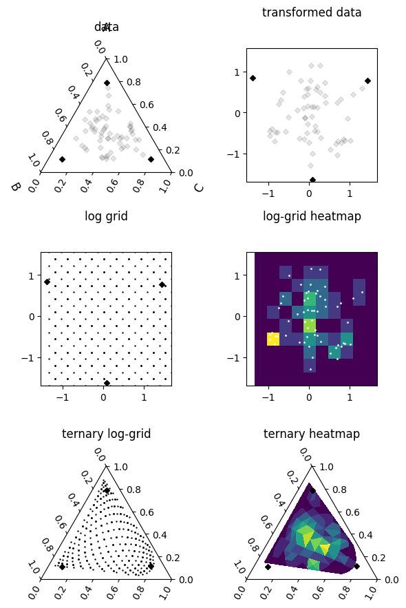
We can see how this works almost exactly the same for the histograms:

coords, H, data = ternary_heatmap(
    df.values,
    bins=10,
    mode="histogram",
    remove_background=True,
    transform=ILR,
    inverse_transform=inverse_ILR,
    grid_border_frac=0.2,
)

fig, ax = plt.subplots(3, 2, figsize=(6, 9))
ax = ax.flat

share_axes([ax[1], ax[2], ax[3]])
ax = axes_to_ternary([ax[0], ax[4], ax[5]])

ax[0].set_title("data", y=1.2)
df.pyroplot.scatter(ax=ax[0], c="k", alpha=0.1)
ax[0].scatter(*data["tern_bound_points"].T, c="k")

ax[1].set_title("transformed data", y=1.2)
ax[1].scatter(*data["tfm_tern_bound_points"].T, c="k")
ax[1].scatter(*data["grid_transform"](df.values).T, c="k", alpha=0.1)

ax[2].set_title("log grid", y=1.2)
ax[2].scatter(*flattengrid(data["tfm_centres"]).T, c="k", marker=".", s=5)
ax[2].scatter(*flattengrid(data["tfm_edges"]).T, c="k", marker=".", s=2)
ax[2].scatter(*data["tfm_tern_bound_points"].T, c="k")

ax[3].set_title("log-grid heatmap", y=1.2)
ax[3].pcolormesh(*data["tfm_edges"], H)
ax[3].scatter(*data["grid_transform"](df.values).T, c="white", alpha=0.8, s=1)

ax[4].set_title("ternary log-grid", y=1.2)
ax[4].scatter(*data["tern_centres"].T, c="k", marker=".", s=5)
ax[4].scatter(*data["tern_edges"].T, c="k", marker=".", s=2)
ax[4].scatter(*data["tern_bound_points"].T, c="k")

ax[5].set_title("ternary heatmap", y=1.2)
ax[5].tripcolor(*coords.T, H.flatten())
ax[5].scatter(*data["tern_bound_points"].T, c="k")

plt.tight_layout()