Geological Timescale

pyrolite includes a simple geological timescale, based on a recent verion of the International Chronostratigraphic Chart [1]. The Timescale class can be used to look up names for specific geological ages, to look up times for known geological age names and to access a reference table for all of these.

[1]

Cohen, K.M., Finney, S.C., Gibbard, P.L., Fan, J.-X., 2013. The ICS International Chronostratigraphic Chart. Episodes 36, 199–204.

First we’ll create a timescale:

from pyrolite.util.time import Timescale

ts = Timescale()

From this we can look up the names of ages (in million years, or Ma):

ts.named_age(1212.1)

'Ectasian'

As geological age names are hierarchical, the name you give an age depends on what level you’re looking at. By default, the timescale will return the most specific non-null level. The levels accessible within the timescale are listed as an attribute:

ts.levels

['Supereon', 'Eon', 'Era', 'Period', 'Superepoch', 'Epoch', 'Age']

These can be used to refine the output names to your desired level of specificity (noting that for some ages, the levels which are accessible can differ; see the chart):

ts.named_age(1212.1, level="Epoch")

'Ectasian'

The timescale can also do the inverse for you, and return the timing information for a given named age:

ts.text2age("Holocene")

(0.0117, 0.0)

We can use this to create a simple template to visualise the geological timescale:

import pandas as pd
import matplotlib.pyplot as plt

fig, ax = plt.subplots(1, figsize=(5, 10))

for ix, level in enumerate(ts.levels):
    ldf = ts.data.loc[ts.data.Level == level, :]
    for pix, period in ldf.iterrows():
        ax.bar(
            ix,
            period.Start - period.End,
            facecolor=period.Color,
            bottom=period.End,
            width=1,
            edgecolor="k",
        )

ax.set_xticks(range(len(ts.levels)))
ax.set_xticklabels(ts.levels, rotation=60)
ax.xaxis.set_ticks_position("top")
ax.set_ylabel("Age (Ma)")
ax.invert_yaxis()

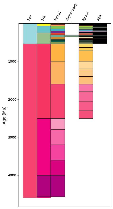
This doesn’t quite look like the geological timescale you may be used to. We can improve on the output somewhat with a bit of customisation for the positioning. Notably, this is less readable, but produces something closer to what we’re after. Some of this may soon be integrated as a Timescale method, if there’s interest.

import numpy as np
from matplotlib.patches import Rectangle

# first let's set up some x-limits for the different timescale levels
xlims = {
    "Eon": (0, 1),
    "Era": (1, 2),
    "Period": (2, 3),
    "Superepoch": (3, 4),
    "Epoch": (3, 5),
    "Age": (5, 7),
}


fig, ax = plt.subplots(1, figsize=(4, 10))

for ix, level in enumerate(ts.levels[::-1]):
    if level in xlims:
        ldf = ts.data.loc[ts.data.Level == level, :]
        for pix, period in ldf.iterrows():
            left, right = xlims[level]
            time = np.mean(ts.text2age(period.Name))
            if ix != len(ts.levels) - 1:
                general_bound = None
                _ix = ix
                while general_bound is None:
                    try:
                        _ix += 1
                        bound_level = ts.levels[::-1][_ix]
                        general_bound = ts.named_age(time, level=bound_level)
                    except IndexError:
                        break
                if bound_level in xlims:
                    _l, _r = xlims[bound_level]
                    if _r > left:
                        left = _r

            rect = Rectangle(
                (left, period.End),
                right - left,
                period.Start - period.End,
                facecolor=period.Color,
                edgecolor="k",
            )
            ax.add_artist(rect)

ax.set_xticks([np.mean(xlims[lvl]) for lvl in xlims.keys()])
ax.set_xticklabels(xlims.keys(), rotation=60)
ax.xaxis.set_ticks_position("top")
ax.set_xlim(0, 7)
ax.set_ylabel("Age (Ma)")
ax.set_ylim(500, 0)

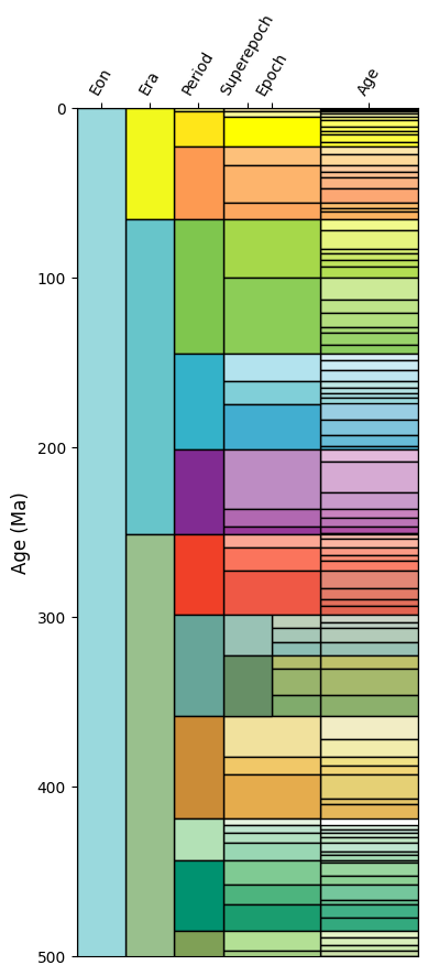
(500.0, 0.0)