Spiderplots & Density Spiderplots
import matplotlib.pyplot as plt
import numpy as np
import pandas as pd
Here we’ll set up an example which uses EMORB as a starting point. Typically we’ll
normalise trace element compositions to a reference composition
to be able to link the diagram to ‘relative enrichement’ occuring during geological
processes, so here we’re normalising to a Primitive Mantle composition first.
We’re here taking this normalised composition and adding some noise in log-space to
generate multiple compositions about this mean (i.e. a compositional distribution).
For simplicility, this is handled by
example_spider_data():
from pyrolite.util.synthetic import example_spider_data

normdf = example_spider_data(start="EMORB_SM89", norm_to="PM_PON")
See also
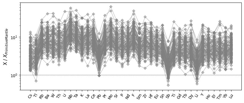
Basic spider plots are straightforward to produce:
import pyrolite.plot

ax = normdf.pyroplot.spider(color="0.5", alpha=0.5, unity_line=True, figsize=(10, 4))
ax.set_ylabel("X / $X_{Primitive Mantle}$")
plt.show()
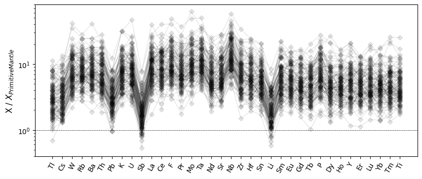
Index Ordering
The default ordering here follows that of the dataframe columns, but we typically
want to reorder these based on some physical ordering. A index_order keyword
argument can be used to supply a function which will reorder the elements before
plotting. Here we order the elements by relative incompatibility (using
pyrolite.geochem.ind.by_incompatibility() behind the scenes):
from pyrolite.geochem.ind import by_incompatibility

ax = normdf.pyroplot.spider(
    color="k",
    alpha=0.1,
    unity_line=True,
    index_order="incompatibility",
    figsize=(10, 4),
)
ax.set_ylabel("X / $X_{Primitive Mantle}$")
plt.show()
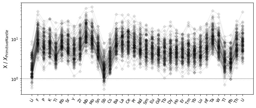
Similarly, you can also rearrange elements to be in order of atomic number:
from pyrolite.geochem.ind import by_number

ax = normdf.pyroplot.spider(
    color="k",
    alpha=0.1,
    unity_line=True,
    index_order="number",
    figsize=(10, 4),
)
ax.set_ylabel("X / $X_{Primitive Mantle}$")
plt.show()
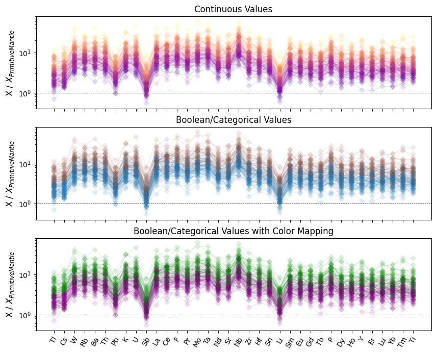
Color Mapping
We can also specify either continuous or categorical values to use for the colors, and even map categorical values to specific colors where useful:
fig, ax = plt.subplots(3, 1, sharex=True, sharey=True, figsize=(10, 8))
ax[0].set_title("Continuous Values")
normdf.pyroplot.spider(
    ax=ax[0],
    unity_line=True,
    index_order="incompatibility",
    cmap="plasma",
    alpha=0.1,
    color=np.log(normdf["Li"]),  # a range of continous values
)
ax[1].set_title("Boolean/Categorical Values")
normdf.pyroplot.spider(
    ax=ax[1],
    alpha=0.1,
    unity_line=True,
    index_order="incompatibility",
    color=normdf["Cs"] > 3.5,  # a boolean/categorical set of values
)
ax[2].set_title("Boolean/Categorical Values with Color Mapping")
normdf.pyroplot.spider(
    ax=ax[2],
    alpha=0.1,
    unity_line=True,
    index_order="incompatibility",
    color=normdf["Cs"] > 3.5,  # a boolean/categorical set of values
    color_mappings={  # mapping the boolean values to specific colors
        "color": {True: "green", False: "purple"}
    },
)
[a.set_ylabel("X / $X_{Primitive Mantle}$") for a in ax]
plt.show()
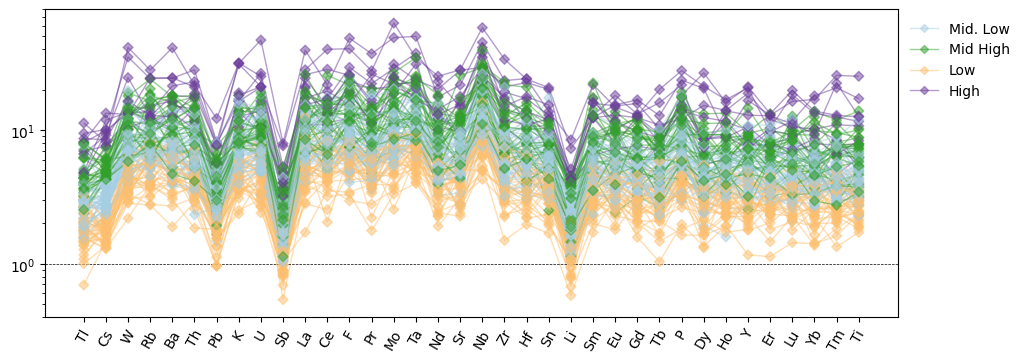
Legend Proxies for Spiderplots
While it’s relatively straightforward to style spider plots as you wish, for the moment can be a bit more involved to create a legend for these styles. Where you’re creating styles based on a set of categories or labels, a few of pyrolite’s utility functions might come in handy. Below we’ll go through such an example, after creating a few labels (here based on a binning of the Cs abundance):
['Mid. Low', 'Mid High', 'Low', 'High']
Categories (4, str): ['Low' < 'Mid. Low' < 'Mid High' < 'High']
Below we’ll use process_color() and
proxy_line() to construct a set of legend proxies.
Note that we need to pass the same configuration to both
spider() and process_color()
in order to get the same results, and that the order of labels in the legend
will depend on which labels appear first in your dataframe or series (and hence the
ordering of the unique values which are returned).
from pyrolite.plot.color import process_color
from pyrolite.util.plot.legend import proxy_line

ax = normdf.pyroplot.spider(
    unity_line=True,
    index_order="incompatibility",
    color=labels,  # a categorical set of values
    cmap="Paired",
    alpha=0.5,
    figsize=(11, 4),
)

legend_labels = pd.unique(labels)  # process_color uses this behind the scenes

proxy_colors = process_color(color=legend_labels, cmap="Paired", alpha=0.5)["c"]

legend_proxies = [proxy_line(color=c, marker="D") for c in proxy_colors]

ax.legend(legend_proxies, legend_labels)
plt.show()
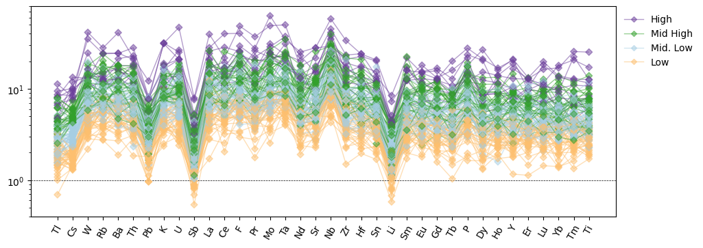
If the specific order of the labels in your legend is important or you only want to include some of the legend entries for some reason, you could use a dictionary to store the key-value pairs and remap the order of the legend entries manually:
proxies = {
    label: proxy_line(color=c, marker="D")
    for label, c in zip(legend_labels, proxy_colors)
}

ordered_labels = ["High", "Mid High", "Mid. Low", "Low"]

ax.legend([proxies[l] for l in ordered_labels], ordered_labels)

plt.show()
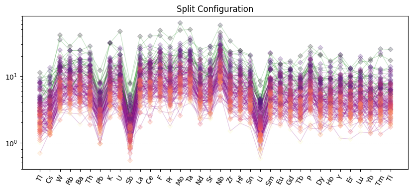
Split Configuration
If you have potential conflicts between desired configurations for the lines and
markers of your plots, you can explictly separate the configuration using the
scatter_kw and line_kw keyword arguments:
fig, ax = plt.subplots(1, 1, sharex=True, sharey=True, figsize=(10, 4))
ax.set_title("Split Configuration")
normdf.pyroplot.spider(
    ax=ax,
    unity_line=True,
    index_order="incompatibility",
    scatter_kw=dict(cmap="magma_r", color=np.log(normdf["Li"])),
    line_kw=dict(
        color=normdf["Cs"] > 5,
        color_mappings={"color": {True: "green", False: "purple"}},
    ),
    alpha=0.2,  # common alpha config between lines and markers
    s=25,  # argument for scatter which won't be passed to lines
)
plt.show()
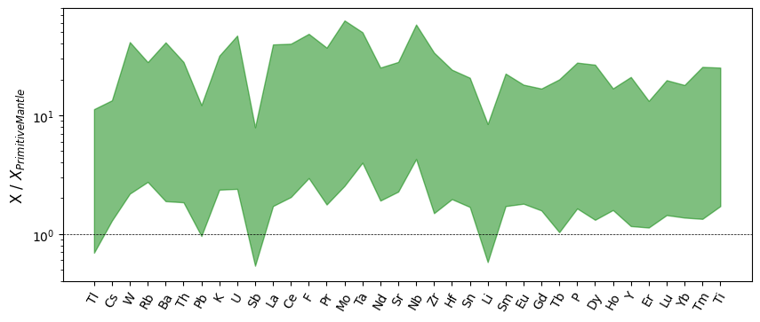
Filled Ranges
The spiderplot can be extended to provide visualisations of ranges and density via the various modes. We could now plot the range of compositions as a filled range:
ax = normdf.pyroplot.spider(
    mode="fill",
    color="green",
    alpha=0.5,
    unity_line=True,
    index_order="incompatibility",
    figsize=(10, 4),
)
ax.set_ylabel("X / $X_{Primitive Mantle}$")
plt.show()
Spider Density Plots
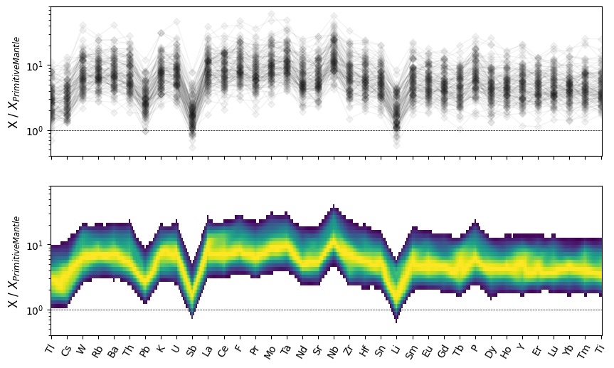
Alternatively, we can plot a conditional density spider plot:
fig, ax = plt.subplots(2, 1, sharex=True, sharey=True, figsize=(10, 6))
normdf.pyroplot.spider(
    ax=ax[0], color="k", alpha=0.05, unity_line=True, index_order=by_incompatibility
)
normdf.pyroplot.spider(
    ax=ax[1],
    mode="binkde",
    vmin=0.05,  # 95th percentile,
    resolution=10,
    unity_line=True,
    index_order="incompatibility",
)
[a.set_ylabel("X / $X_{Primitive Mantle}$") for a in ax]
plt.show()
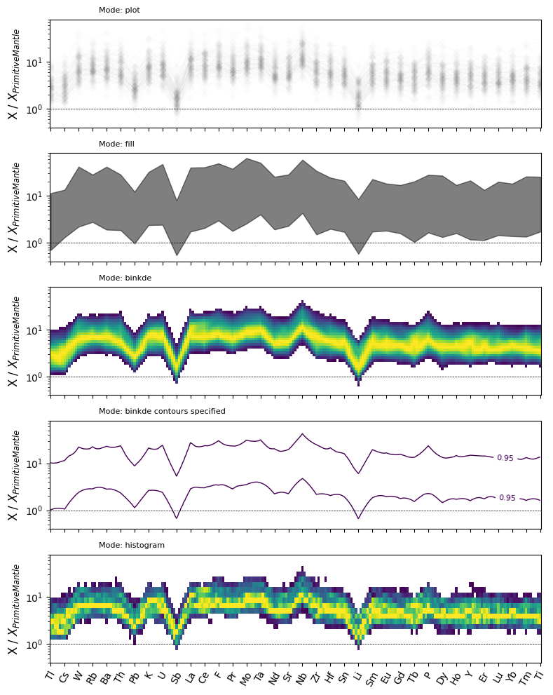
We can now assemble a more complete comparison of some of the conditional density modes for spider plots:
modes = [
    ("plot", "plot", [], dict(color="k", alpha=0.01)),
    ("fill", "fill", [], dict(color="k", alpha=0.5)),
    ("binkde", "binkde", [], dict(resolution=5)),
    (
        "binkde",
        "binkde contours specified",
        [],
        dict(contours=[0.95], resolution=5),  # 95th percentile contour
    ),
    ("histogram", "histogram", [], dict(resolution=5, bins=30)),
]
down, across = len(modes), 1
fig, ax = plt.subplots(
    down, across, sharey=True, sharex=True, figsize=(across * 8, 2 * down)
)
[a.set_ylabel("X / $X_{Primitive Mantle}$") for a in ax]
for a, (m, name, args, kwargs) in zip(ax, modes):
    a.annotate(  # label the axes rows
        "Mode: {}".format(name),
        xy=(0.1, 1.05),
        xycoords=a.transAxes,
        fontsize=8,
        ha="left",
        va="bottom",
    )
ax = ax.flat
for mix, (m, name, args, kwargs) in enumerate(modes):
    normdf.pyroplot.spider(
        mode=m,
        ax=ax[mix],
        vmin=0.05,  # minimum percentile
        fontsize=8,
        unity_line=True,
        index_order="incompatibility",
        *args,
        **kwargs,
    )

plt.tight_layout()
/home/docs/checkouts/readthedocs.org/user_builds/pyrolite/checkouts/develop/pyrolite/plot/spider.py:211: UserWarning: No data for colormapping provided via 'c'. Parameters 'vmin' will be ignored
  ax.scatter(
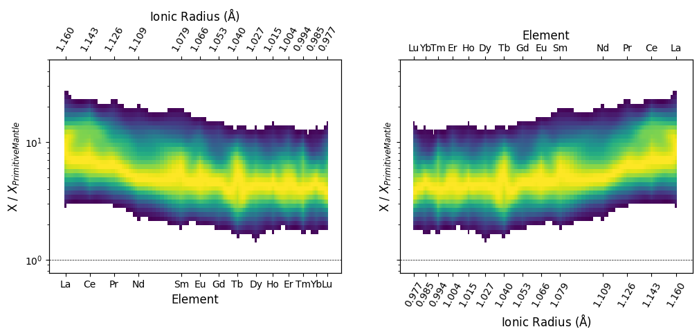
REE Density Plots
Note that this can also be used for REE-indexed plots, in both configurations. Here we first specify a set of common keyword-argument configurations and use them for both plots:
REE_config = dict(unity_line=True, mode="binkde", vmin=0.05, resolution=10)

fig, ax = plt.subplots(1, 2, sharey=True, figsize=(12, 4))
normdf.pyroplot.REE(ax=ax[0], **REE_config)
normdf.pyroplot.REE(ax=ax[1], index="radii", **REE_config)
[a.set_ylabel("X / $X_{Primitive Mantle}$") for a in ax]
plt.show()
See also
Total running time of the script: (0 minutes 3.962 seconds)